Cardinality Estimation is one of the hidden gems in SQL Server. In general, Cardinality Estimation means that the Query Optimizer tries to find out during the query compilation, how many rows – on average – are returned from the various operators in the Execution Plan. This estimation is used to drive the plan generation itself and choose the right plan operators – for example a physical join operator like Nested Loop, Merge Join, or Hash Join. When these estimates are wrong, then the Query Optimizer will choose a wrong plan operator, and your query can be veeeeeeery slow – trust me! 😉
The Query Optimizer uses for the Cardinality Estimation the so-called Statistic objects. Every time when you create an Index, SQL Server also creates an underlying Statistic object. That object describes the data distribution of that index. In addition, SQL Server is also able to create statistic objects during query execution, when necessary (Auto Create Stats). The data distribution itself (of the first column in a composite index key) is described in a so-called Histogram.
One of the main pains of the Histogram is it can only have up to 200 so-called Steps. A step describes the data distribution for a given part of your column data. The larger your table gets, the more inaccurate your histogram will be, because you can only have up to 200 steps (a histogram must be as compact as possible, it must fit onto one page of 8kb).
For additional columns in a composite index key, SQL Server stores in the statistics object a so-called Density Vector that describes how unique the values of the composite index keys are (in combination to each other). When you have – for example – 3 different values in a column, the density vector of that column is 0.33333 (1 divided by 3).
Beginning with SQL Server 2008, SQL Server also supports so-called Filtered Statistics (along with Filtered Indexes). With Filtered Statistics you can create a statistic objects across a subset of your data. For that subset of data, you are getting again a Histogram, and the Density Vector. If you have outliers in your data, you can create a Filtered Statistics object for that range to give the Query Optimizer a better estimation how many rows are returned, when that specific area of your data is queried. So you are just improving the Cardinality Estimation with Filtered Statistics that will give you directly a better performing Execution Plan. The following listing shows a simple example how a Filtered Statistics object is created in SQL Server 2008 and onwards:
CREATE STATISTICS Country_Austria ON Country(ID)
WHERE Name = 'Austria'
GO
As you can see from the listing above, you just restrict with the WHERE clause the subset of the table data, that should be described through the new Filtered Statistics object. But the Query Optimizer can only make use of this new statistics object, when you also include the *same* WHERE clause in your query, like:
SELECT SalesAmount FROM Country
INNER JOIN Orders ON Country.ID = Orders.ID
WHERE Name = 'Austria'
GO
If the same WHERE clause is not included in your query, the Query Optimizer will use the default statistics object that comes along with the index that is accessed in the Execution Plan. If you enable the Trace Flag 9204 for the previous query, you can also see which statistics where used by the Query Optimizer during the Cardinality Estimation:
SELECT SalesAmount FROM Country
INNER JOIN Orders ON Country.ID = Orders.ID
WHERE Name = 'Austria'
OPTION
(
    RECOMPILE,-- Used to see the Statistics Output
    QUERYTRACEON 3604,-- Redirects the output to SSMS
    QUERYTRACEON 9204 -- Returns the Statistics that were used during Cardinality Estimation ("Stats loaded")
)
GO
The query itself must be also compiled (hence the query hint RECOMPILE, if an Execution Plan is already cached), so that you can see in the messages window of SQL Server Management Studio the Statistics that were used for the Cardinality Estimation.
Based on this simple introduction to Filtered Statistics, I want to show you now a real world example how Filtered Statistics can improve the quality of the Execution Plan. In the first step we are creating 2 tables: Country and Orders. The Country table is a simple lookup table, where I have stored all the countries where I’m doing business. And the Orders table just tracks every order, and has a relationship to the Country table so that I know in which country that order was placed. In a Data Warehouse scenario you can also think about a fact and dimension table.
-- Create a new database
CREATE DATABASE FilteredStatistics
GO

-- Use it
USE FilteredStatistics
GO

-- Create a new table
CREATE TABLE Country
(
ID INT PRIMARY KEY,
Name VARCHAR(100)
)
GO

-- Create a new table
CREATE TABLE Orders
(
ID INT,
SalesAmount DECIMAL(18, 2)
)
GO
In the next step I’m creating a supporting Non-Clustered index on the column Name of the table Country, and I’m also creating a Clustered Index on the columns ID, and SalesAmount of the table Orders:
-- Create a Non-Clustered Index
CREATE NONCLUSTERED INDEX idx_Name ON Country(Name)
GO

-- Create a Clustered Index
CREATE CLUSTERED INDEX idx_ID_SalesAmount ON Orders(ID, SalesAmount)
GO
And finally I’m inserting my initial data in both tables:
-- Insert a few records into the Lookup Table
INSERT INTO Country VALUES(0, 'Austria')
INSERT INTO Country VALUES(1, 'UK')
INSERT INTO Country VALUES(2, 'France')
GO

-- Insert uneven distributed order data
INSERT INTO Orders VALUES(0, 0)

DECLARE @i INT = 1

WHILE @i <= 1000
BEGIN
INSERT INTO Orders VALUES (1, @i)
SET @i += 1
END
GO
To make sure that all statistics are up-2-date, I’m updating the statistics with a full scan:
-- Update the Statistics on both tables
UPDATE STATISTICS Country WITH FULLSCAN
UPDATE STATISTICS Orders WITH FULLSCAN
GO
Let’s run now the following query:
SELECT SalesAmount FROM Country
INNER JOIN Orders ON Country.ID = Orders.ID
WHERE Name = 'UK'
OPTION
(
RECOMPILE,-- Used to see the Statistics Output
    QUERYTRACEON 3604,-- Redirects the output to SSMS
    QUERYTRACEON 9204-- Returns the Statistics that were used during Cardinality Estimation ("Stats loaded")
)
GO
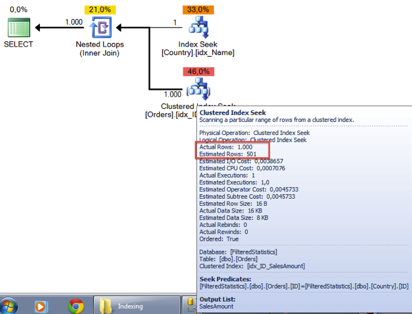
When you look in the Execution Plan, you can see that we have a big problem with the Cardinality Estimation:

SQL Server estimates 501 rows, and in reality the Clustered Index Seek operator returns 1000 rows. SQL Server uses here the Density Vector of the Statistics Object idx_ID_SalesAmount to make that estimation: the Density Vector is 0.5 (we have only 2 distinct values in that column), and therefore the estimation is 501 (1001 * 0.5).
When you run the same query again, with a parameter value of “Austria”, SQL Server will again estimate 501 rows, but the query itself will only return 1 row… This behavior can have a huge negative side effect in the Execution Plan, when other operators are using these estimations for their operation. For example, a Sort and Hash Operator uses these estimations to size the needed memory grant accordingly. If you have an Under-Estimation, your query will spill over to TempDb, if you have an Over-Estimation, you are just wasting memory, which can also lead to contention problems, when you have a huge amount of concurrent queries (the maximum amount of Query Memory is restricted by Resource Governor…)
You can help in that specific scenario with a Filtered Statistics object. This will give SQL Server more information about the data distribution itself, and will also help in the Cardinality Estimation. For that specific scenario, I have created 2 different Filtered Statistics, for every country (where I had sales) I have created a separate Filtered Statistics object:
-- Fix the problem by creating Filtered Statistics Objects
CREATE STATISTICS Country_UK ON Country(ID)
WHERE Name = 'UK'

CREATE STATISTICS Country_Austria ON Country(ID)
WHERE Name = 'Austria'
GO
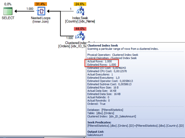
When you are now rerunning the query, you can finally see that the Cardinality Estimation is correct:

When you have created Filtered Statistics on your tables, you also have to be aware about the maintenance. The automatic maintenance is again done by SQL Server when 20% of the underlying data has changed - from the *whole* table itself!!! Imagine you have a table with 10000 rows, and you have created a Filtered Statistics object on a subset of that table, let’s say 500 records. In that case, SQL Server will update the Filtered Statistics object when around 2000 data changes where done for the given columns. So you have to change 4x the data in the Filtered Statistics objects, until SQL Server will invalidate and update it (when you have no data changes outside the Filtered Statistics interval). So this is a big bummer, that you have to have in your mind, when you are working with Filtered Statistics.
I hope that this blog posting gave you a good overview about Filtered Statistics, and how you can use them in SQL Server to improve the Cardinality Estimation for given queries.
Thanks for reading
-Klaus